
The Closure Problem: When Going Up Forces Something to Come Down
Pick up any whole-rock geochemistry dataset. The columns will be SiO2, Al2O3, FeO, MgO, CaO, Na2O, K2O, TiO2, MnO, P2O5, and a handful of trace elements. Sum the major-oxide row. You will get something extremely close to 100. That is not a coincidence. It is the lab forcing the columns to add up, on the (correct) view that an oxide analysis whose components don't add up to a hundred percent has measurement errors somewhere. Closure is part of how the data exists at all.
It is also a persistent source of trouble in geochemical statistics, and has been recognised as one since at least the 1960s. The reason is straightforward. If your row has to sum to 100, then making any one component bigger forces at least one other component to be smaller. There is nowhere else for the percentage to go. The components are linked by the constraint, and that link shows up in every correlation, regression, principal component, and clustering result you compute on the raw percentages.
The arithmetic, in one figure
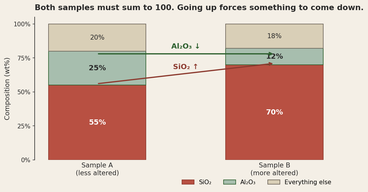
Look at sample B. SiO2 went up by 15 percentage points relative to sample A. Something had to give that 15 back, and Al2O3 gave back 13 of them. If you had a thousand samples like these and you computed the Pearson correlation between SiO2 and Al2O3, you would find a strong negative correlation. You would write a paragraph about how silica enrichment is associated with alumina depletion. The paragraph would be wrong. There may also be a real geochemical relationship, but you cannot tell, because the closure constraint is producing a spurious negative correlation regardless of whether anything geological is happening at all.
The same data, before and after closure
The cleanest way to see this is to simulate it. I generated 250 hypothetical rocks where the absolute amounts of SiO2, Al2O3, and "everything else" are statistically independent. Then I closed the data to 100 percent, the way a lab would, and looked at the resulting correlation.
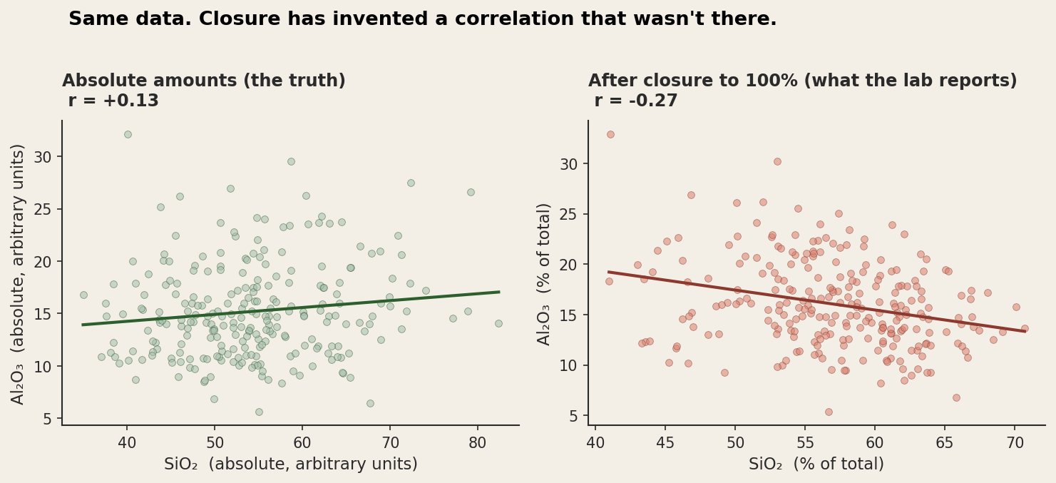
The "absolute" panel is the truth. SiO2 and Al2O3 are statistically independent here, by construction. The correlation is essentially zero. The "closed" panel is what comes back from the lab. Same samples, same underlying world, but now the correlation is meaningfully negative. The spurious correlation is a property of the analysis pipeline, not a property of the rocks.
This is not a contrived demonstration. Karl Pearson noticed this in 1897, in a paper with the marvellous title "Mathematical Contributions to the Theory of Evolution.—On a Form of Spurious Correlation Which May Arise When Indices Are Used in the Measurement of Organs." He was looking at bone-length ratios, but the math is identical, and the closure problem in geochemistry is just one corner of a larger family.
The same two elements, two different correlations
Closure does something stranger than manufacture a spurious correlation. It makes the correlation refuse to hold still.
Two geologists analyse the same rocks. They are interested in the same two oxides — say Al2O3 and CaO. The first computes the correlation across a full ten-oxide dataset. The second drops the minor oxides and works with a six-oxide subset. They get different correlation coefficients. Not slightly different — different enough to flip sign. One reports a positive relationship, the other a negative one. Same rocks. Same two elements. Same samples. Both did the arithmetic correctly.
The correlation between two parts of a composition is not a property of those two parts. It is a property of the entire set of parts you chose to put in the table. Add a variable or remove one, and every remaining correlation can shift, because closure renormalises across whatever is present. This is called subcompositional incoherence, and it has no equivalent in unconstrained data. The correlation between height and weight does not care whether you also measured shoe size. The correlation between two oxides cares enormously about what else is in the spreadsheet.
So the honest answer to "are these two elements correlated" is a question in return: correlated within what? Until you specify the whole composition, there is no single correct number. That is the part that earns the word paradox. It is not that the statistics are hard. It is that the quantity you were trying to measure does not exist in the form you assumed. Log-ratios fix this too — ratios between specified parts stay coherent when the rest of the table changes, which is much of why Aitchison built the framework around them — but you have to know the problem is there before the fix means anything.
The simplex, and why this is geometry not algebra
The deepest version of the problem is geometric. Every three-component composition lives somewhere on a triangle. Every four-component composition lives somewhere inside a tetrahedron. In general, every D-component composition lives on a (D-1)-dimensional triangular surface called a simplex. Standard statistical tools, including Pearson correlation, ordinary least squares, principal component analysis, k-means, and almost everything else in your toolkit, assume the data lives in ordinary Euclidean space, where the dimensions are independent and you can move freely in any direction. Compositional data does not. It lives on the simplex, and the simplex has very different geometric properties.
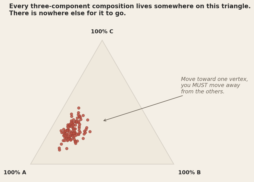
This is John Aitchison's contribution. In a 1982 paper, Aitchison pointed out that compositional data lives in a fundamentally different geometric space and proposed the family of log-ratio transforms (centred log-ratio, or CLR; isometric log-ratio, or ILR; additive log-ratio, or ALR) that map the simplex into ordinary Euclidean space, where the standard tools actually work. The correlation, regression, or PCA you run on the log-ratios is not "a CLR-friendly version of the analysis you wanted." It is the analysis you wanted, finally being run on data that satisfies the assumptions of the method. The raw-percentage version was the broken one all along.
The geological response to this has been spotty. Pearce element ratios (Pearce, 1968) tackled the problem in igneous petrology by using ratios anchored to a conserved element. Isocon analysis (Grant, 1986) does the same for alteration studies, by identifying immobile elements that can be used to back out absolute mass changes from relative-percentage data. Both methods are, in their own ways, ways of escaping the simplex without going through Aitchison's full machinery, and both work well for the specific problems they were designed for. For general geostatistics, though, the modern answer is the log-ratio transform, and it matters more as machine-learning workflows become routine in exploration. A model trained on raw oxide percentages inherits every closure artifact in the data, and can end up learning the constraint itself instead of the geology. It is an easy step to skip in a pipeline, and a hard one to notice you skipped.
Where this hides in real geoscience workflows
It hides in more places than you'd think.
Whole-rock major-element correlations are the canonical case. Any pairwise correlation you compute on weight-percent oxides is contaminated by closure. Bivariate plots of MgO versus SiO2 in basalts look like fractionation trends, and there really is fractionation happening, but the slope you measure is partly fractionation and partly the constraint that going up in one forces the other down. Disentangling the two requires either a log-ratio transform or knowledge of an immobile reference element.
Alteration studies are the case where this hurts most. The whole point of an alteration study is to ask "what mass changes have happened relative to the unaltered protolith?" If your data is in weight percent, you cannot answer this question, because the percentages renormalise after every gain or loss. A rock that has gained 30 percent silica by mass and lost nothing else will show, after closure to 100 percent, a relative decrease in everything else, including the elements that didn't go anywhere. The mobile-element story and the closure story become indistinguishable. Grant's isocon method exists precisely to handle this.
Element-ratio diagrams are a partial solution that introduce their own demons. Ratios remove some of the closure pathology but inflate variance dramatically, especially when the denominator is small. The Cu/Zn ratio at low Zn is wild. The Ishikawa Alteration Index (K2O+MgO over K2O+MgO+CaO+Na2O) is a ratio of compositional sums, which makes it both partly closure-immune and noisy, depending on which way the underlying mobility went.
REE patterns are normalised compositions by construction. The chondrite-normalised REE pattern of a sample sums (over the rare-earths) to whatever it sums to, and the differences between samples are conventionally displayed on a log scale. That convention exists mainly for readability, since REE abundances span orders of magnitude, but it does real statistical work as well: plotting in logs is already most of the way to a log-ratio. A sound convention that holds up for more reasons than it was adopted for.
Modal mineralogy sums to 100 by definition. If you compute correlations between modal abundances of plagioclase and quartz across a granite suite, you will find a robust negative correlation, and most of it will be closure rather than petrology. The same is true of QEMSCAN data, automated mineralogy reports, and any other "fraction of total" output.
The data-science angle, which turns out to be everywhere
Compositional data is everywhere in modern data science. It is rare for anyone to call it that, but the math is the same and the failure modes are the same.
Microbiome data. Sequencing reads are converted to relative abundances of microbial taxa. Those abundances sum to one. Every correlation between two taxa across a sample set is contaminated by closure. The microbiome literature has been quietly catching up to compositional methods for the better part of the last decade.
Document-term frequencies. The bag-of-words representation of a document, normalised by total word count, is a composition over the vocabulary. Topic modelling that works on raw frequencies has the same closure issues. Latent Dirichlet Allocation handles this elegantly because it models compositions natively (the Dirichlet distribution is a distribution over the simplex), but ad hoc normalisation pipelines that go straight from term counts to cosine similarity are flying blind.
Image colour histograms. The fraction of pixels in each colour bin is a composition. Distance between images computed naively on these histograms is distance in the simplex, treated as if it were Euclidean.
Market shares, voting splits, time-allocation surveys, budget allocations. All of these sum to a constant. All of them have been the subject of statistical analyses that assumed Euclidean geometry. All of those analyses are, to varying degrees, contaminated by closure.
Softmax outputs of any classifier. The probability vector that a neural network returns is a composition over classes. Computing distances or correlations between softmax outputs in the usual Euclidean way is the same kind of mistake. KL divergence is the right notion of distance here, and it is, not coincidentally, intimately related to log-ratio transforms.
The general lesson is that a constraint of the form "these features sum to a constant" is not innocent bookkeeping. It is a hard geometric constraint on what your data can look like, and it has consequences for every statistic you compute. The sooner you notice you are dealing with a composition, the sooner you can stop doing standard statistics on it and start doing the right ones.
What to actually do
Notice when your data is compositional. The signature is "the rows sum to a constant." That constant is usually 1, 100, or "approximately 100." If you see it, you have closure. Not "you might have closure"; you have it.
Work in log-ratio space when you can. The centred log-ratio (CLR) transform takes a row of percentages, divides each entry by the geometric mean of the row, and takes logs. The result is unbounded, behaves like Euclidean data for most purposes, and supports the standard statistical toolkit. Aitchison's Statistical Analysis of Compositional Data (1986) is still the canonical reference. The Python library pyrolite and the R package compositions implement the transforms cleanly.
The closure problem is a matter of degree. Strictly, every concentration is a fraction of the whole rock, so ppm data is compositional too — a million ppm is the entire sample. But the constraint only bites hard under two conditions: the parts have to be large, and the lab has to have renormalised them as a set. Major elements meet both. They are reported as oxides closed to 100 percent, and each one is a big enough slice that moving it genuinely forces the others down. Trace elements meet neither. They are measured independently, not renormalised against one another, and each is such a small fraction of the rock that when one goes up, the compensation is absorbed by the major-element matrix rather than by the other trace elements. So a Pearson correlation between two trace elements is not perfectly closure-free, but it is usually close enough to honest to use. Between two major oxides, it is not.
For alteration work, use isocon analysis. Identify an immobile reference element (Zr, Ti, Al2O3 in some settings), compute mass-balance ratios relative to that reference, and read off real gains and losses. Grant (1986) is the standard and is mercifully short.
Be especially careful with PCA on raw oxides. The first principal component of a closed dataset is almost always dominated by the closure constraint itself. The "PC1 controls SiO2 versus everything else" story is partly geology and partly arithmetic, and you cannot tell which is which without going to log-ratios first.
If you must do correlation on closed data, report what you did. Saying "we use raw weight-percent oxides; results are subject to closure effects" is much better than letting the reader assume the analysis was clean. Ideally you also do the log-ratio version and compare.
The closure problem is the geochemist's first ghost in the same way that selection bias is the epidemiologist's. It haunts the data not because anyone made a mistake, but because the way the data exists at all imposes a constraint that the standard statistical tools were never designed to honour. The fix is not to ignore the ghost. It is to learn its rules and work around them.
In a dataset that has to add up to a hundred, nothing moves alone; so be slow to trust any correlation that assumes it does.