
Berkson's Paradox: Why Your Best Samples Lie to You
There is a strange statistical pattern in NBA data. Among professional players, shorter athletes tend to jump higher than taller ones. Take a moment with that. Do shorter people have unusually springy legs? It is worth thinking about why before reading on, because the answer is also why many exploration geochemistry datasets quietly mislead the people analyzing them.
The puzzle is real. If you correlate height against vertical leap inside the NBA, you get a negative trend. Outside the NBA, in the general population of adults, the same two variables are essentially uncorrelated. Tall people are not, on average, worse jumpers than short people. Something happens in the act of becoming an NBA player that creates a relationship that does not exist in the underlying population.
That something is Berkson's paradox. It is one of the most under-appreciated traps in applied statistics, and it shows up in geological datasets more often than people realize.
What is actually happening in the NBA
To make it into the NBA, a player needs to be exceptional at basketball. Roughly speaking, you can think of basketball ability as a product of athletic traits: height, leaping, speed, coordination, court vision, shooting touch, and more. The league does not care which combination gets you there. It only cares that the total is high enough.
That means a 7'1" player can be in the league with a relatively modest vertical leap, because their height alone makes them valuable. A 6'0" player has to be an extraordinary athlete in every other dimension to compensate. Average jumpers who are also average height never make the league at all.
The NBA filter is essentially: height x jumping x (other skills) > some threshold. Once you condition on that filter, the remaining players show a negative correlation between height and jumping, even though the two traits are independent in the general population. The shorter players you see in the league are biased toward being amazing jumpers. The taller players are biased toward not needing to jump as much.
Why product, not sum
It is worth pausing on the multiplication for a moment, because it changes how you should think about the filter. If basketball ability were a sum, then enough jumping ability could in principle make up for anything. A 5'4" player with a transcendent vertical could still clear the threshold. The arithmetic would allow it.
That is not how the NBA actually works. A 5'4" player is a zero on the height axis, and zero times anything is zero. No amount of leaping ability rescues a frame that small. The other factors do not add to height; they multiply with it. Each one acts as a gate. Drop any one of them too low and the product collapses regardless of the others.
That is the structure that produces exceptional outcomes in most domains. Truly remarkable performance usually requires several traits to all be at least pretty good, and at least one to be outstanding. It is rarely about being magnificent on a single axis while flatlining on the others. The selection filter is multiplicative, and the same logic shows up everywhere it matters.
Geologists already think this way, even if they do not call it that. The Mineral Systems Approach is essentially a product. A deposit needs a source, a pathway, a trap, a depositional mechanism, and enough preservation to still be there when we go looking. Knock any one of those to zero and the system fails. A spectacular source with no pathway gives you nothing. A perfect trap with no fluids gives you nothing. The ingredients multiply.
Berkson's paradox arises in product-like filters even more cleanly than in sum-like ones. The lower-left corner of the plot, where both traits are weak, does not just get clipped off. It gets carved out in an L-shape, because failing on either axis is enough to keep you out. That carved-out shape is what produces the negative correlation in the survivors.
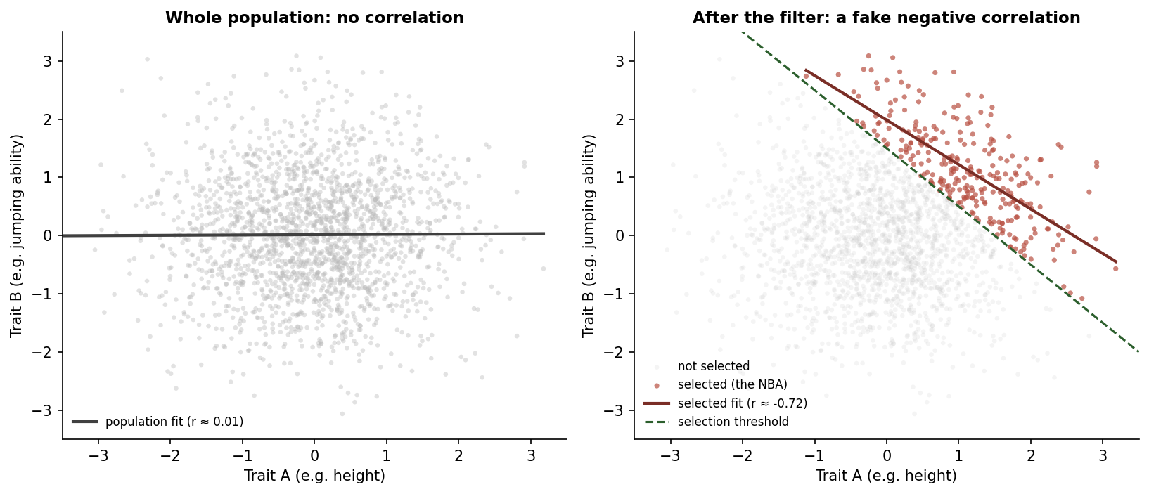
Notice how clean the effect is. There is no underlying relationship between the two traits. The negative slope on the right is created entirely by the selection rule. The threshold cuts off the lower-left corner of the plot, and that asymmetric removal is what makes the remaining points line up diagonally.
Berkson's paradox in one sentence. When inclusion in a dataset depends on the product (or any combination) of two variables exceeding a threshold, those variables can appear negatively correlated in the dataset even when they are independent or positively correlated in the underlying population.
The dual-talent students
The same effect shows up in education. There is a long-running observation that, among students at selective universities, the ones who are strong in math tend to be weaker in English and vice versa. People reach for explanations like "the brain specializes" or "you are either a math person or a language person."
Both stories are mostly wrong. In the broader applicant pool, math and English ability are weakly positively correlated. Students who are strong in one tend to be at least decent in the other.
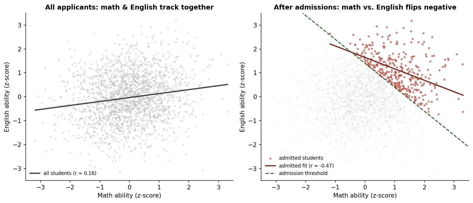
Once you condition on admission to a selective school, the same pattern as the NBA appears. A student admitted with mediocre English scores almost certainly has exceptional math scores, because something had to get them through the gate. A student admitted with mediocre math scores almost certainly has exceptional English. The students who are average at both never made it into the dataset.
So the classroom observation that "people are good at one or the other" is really an observation about the admissions filter. The filter makes students look like specialists, when in reality most of them are just exceptional in at least one direction. The trade-off appearance is geometry, not biology.
Now think about your geochemistry database
This is where it stops being abstract.
Imagine all the rock in a province. Most of it is unremarkable. Background concentrations of pathfinder elements, subtle geochemical variability, very little of geological interest at the scale we usually care about. In the actual rock, two pathfinder elements like Cu and Au tend to be weakly positively related, because both can be elevated by the same kinds of geological processes (fluid flow, sulfide concentration, alteration overprint).
Now think about which of those rocks ends up in an assay database.
A sample is collected and submitted for analysis if a geologist thought it was worth looking at. Maybe there was visible mineralization, alteration, a textural feature, an interesting structural setting, or a previous result nearby. Lab budgets are finite, so triaging is real. Even when entire holes are sampled at fixed intervals, those holes were drilled where someone already saw something. Historical assessment work tends to focus on showings. Public databases often inherit decades of those decisions.
What that means in practice is that a sample tends to make it into the analyzed dataset if it scored high on at least one geological criterion. High Cu, or high Au, or visible sulfide, or mapped alteration, or favourable host. That is an "OR" filter, and an "OR" filter is exactly what creates Berkson's paradox.
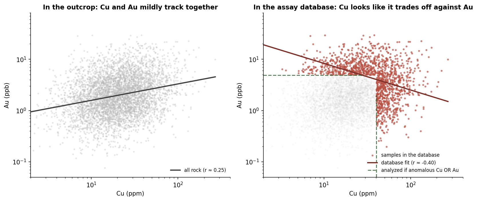
The right-hand panel is the database an exploration team actually works with. The left-hand panel is the geological reality the database is supposed to represent. They tell genuinely different stories about the relationship between Cu and Au. And the team only ever sees the right-hand panel.
If you fit a model on the database without thinking about the filter, you might conclude that Cu and Au are antagonistic. You might engineer features that penalize their co-occurrence. You might dismiss a target where both are moderately elevated as unimpressive, because the database has trained your intuition to expect one or the other. None of those conclusions follow from the actual rock. They follow from the way the rock got into the dataset.
Why the analyzed samples are the NBA stars
Here is the analogy. The samples in your assay database are the league. They earned their way in by being unusually interesting on at least one axis. The mass of unremarkable rock that surrounds the deposit, the in-between samples that nobody bothered to send to the lab, those are the general population. They are the people who never tried out for the NBA.
And, just like the NBA, the relationships you observe inside the league do not generalize to the population it was drawn from. The shorter NBA players are exceptional jumpers because the filter required it. The lower-Cu samples in your database are exceptional in Au because the filter required it. The geometry is the same.
The practical takeaway. Most exploration databases are not random samples of rock. They are filtered collections of samples that passed at least one anomaly test. Correlations within those collections describe the filter as much as the geology.
What to do about it
Berkson's paradox is not a reason to throw out exploration data. The samples are still real. The assays are still real. What changes is how you interpret patterns within them.
A few habits help. First, separate the question of what is in the rock from the question of what is in the database. They are not the same. Statements about the database should be qualified as such, especially when the conclusion involves a correlation or trade-off.
Second, think about the selection process explicitly. What filter caused this sample to be analyzed? Was it a routine grid, a follow-up on an anomaly, a step-out on a known showing, or a historical assessment program with its own logic? Different filters produce different Berkson distortions, and not knowing the filter is its own form of bias.
Third, where it matters, complement the targeted database with something closer to a representative sample. Reconnaissance grids, regional geochemistry surveys, and routine sampling along entire holes (not just the visibly interesting intervals) can act as a control. The pattern you see in the targeted dataset is more trustworthy if it survives in the unfiltered one.
Fourth, when training machine learning models, be careful about what your training data actually represents. A prospectivity model trained only on samples near known deposits is learning the structure of the discovery process, not the structure of the rock. That can still be useful, but it is a different model than the one most people think they are building.
The wider point
Berkson's paradox is one example of a more general issue: every dataset has a story about how it came to exist, and that story shapes what the data can and cannot say. In exploration, the story is rarely "we sampled the earth at random." It is almost always "we sampled where we thought it was worth sampling." That is a sensible way to allocate budget. It is a difficult way to estimate background relationships.
The geologists who are best at applied statistics are not necessarily the ones who know the most tests. They are the ones who pause and ask, before any analysis, what filter produced the data on the desk in front of them.
Further reading
If you want to read more on Berkson's paradox in different settings, a few good entry points:
- Allen Downey's Probably Overthinking It, which is where the NBA and dual-talent examples in this post come from. The book is a careful tour of the kinds of statistical illusions that show up in real datasets.
- The Wikipedia article covers the original epidemiological setting and the canonical celebrity-talent illustration.
- The Brilliant.org wiki entry walks through the GPA versus SAT example with a clean visualization.
The data on your desk is not the rock in the ground. It is the rock that earned its way into the dataset. Knowing the difference is most of the work.
Inside any selected sample, the most interesting correlations are often the ones that were created by the selection itself.