
Survivorship Bias: The Drivers You Never See
Think about the last drive you took on the highway. Now think about the drivers you noticed. There were the ones who blew past you in the left lane (idiots, obviously). There were the ones you slowly caught up to and overtook (also idiots, but in the other direction). What about everyone else?
Here is the strange thing. The drivers whose speed was within a few kilometres of yours basically never enter your awareness. You don't pass them. They don't pass you. You drift along at roughly the same pace for kilometres, and they are utterly invisible to you. The only drivers you ever actually encounter as drivers are the ones moving at a different speed than you are. Faster, slower, never the same.
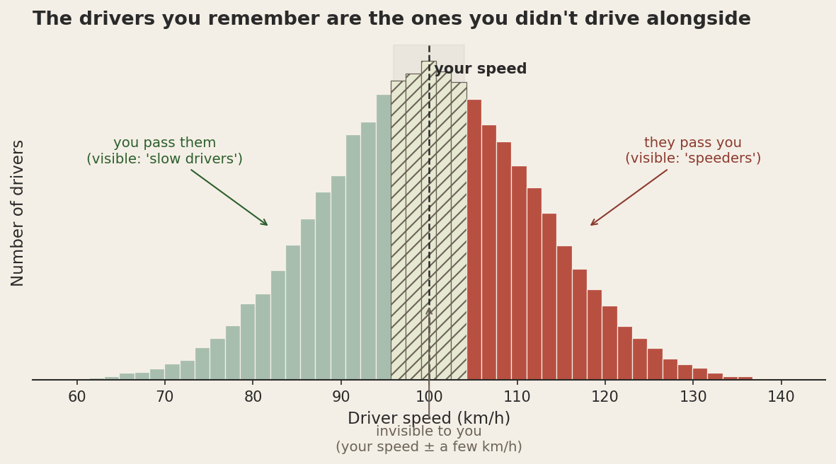
The result is that every commute trains you on a biased sample. The bell curve of actual driving speeds is wide and roughly symmetric. Your perceived sample of "drivers I noticed today" has an enormous hole punched in the middle of it, exactly where most drivers actually live. From your seat, the road looks bimodal. There are speed demons and there are slowpokes, and apparently nobody drives sensibly except you.
This is survivorship bias, and traffic teaches it more cleanly than airplanes do, because the missing data isn't even gone. It's right there. It's just not visible to you, because the filter that makes a driver visible to you (relative motion) systematically excludes the population you most need to see.
Why we keep telling the airplane story instead
The classic story goes like this. In 1943, the U.S. Navy looked at bullet hole patterns on bombers returning from missions over Europe and concluded they should add armour where the holes were densest, on the wings and rear fuselage. Abraham Wald, a statistician at the Statistical Research Group, told them they had it exactly backwards. The planes that came back were the ones that could survive being hit there. The ones that took fire in the engines and cockpit didn't make it home to be measured. Armour the unhit zones, he said. The undamaged areas of the surviving planes are the lethal areas of the dead ones. (For the canonical bullet-hole diagram, see the Wikipedia entry on survivorship bias.)
It is a beautiful story. It also has the shape of a finished proof, and that is the problem with it as a teaching example. The missing planes are obviously gone. They crashed. Nobody is confused about whether the dataset is complete; the dataset is literally physical wreckage at the bottom of the English Channel. Once Wald points this out, the move feels obvious in retrospect.
The traffic version is harder, and that is what makes it the better teacher. Nothing crashed. Nothing is missing. The drivers who match your speed are out there, on the same road, in the same data-generating process. They are just invisible to your particular sampling mechanism. You are not missing data; you are oversampling the tails. That feels different from Wald's case, but mathematically it is the same problem with a different filter.
Where this hides in exploration
If you have spent any time around mineral exploration, you have probably read more papers about Olympic Dam and Sudbury and Voisey's Bay than you can remember. You have heard the structural setting of the Carlin Trend explained in a dozen short courses. You have seen the alteration zonation of Pebble or Bingham Canyon redrawn so many times that you could reproduce it from memory. There are textbook chapters, classification schemes, ore deposit models, and decades of literature on these systems.
You have heard much less about the prospects that drilled out at three metres of one g/t and were quietly abandoned. You have heard nothing about the geochemical anomalies that were never followed up because the field season ended. You have heard nothing at all about the deposits under cover that nobody has yet found. This is not because anyone is hiding anything. It is the same filter as the highway. The visible cases are the ones that moved at a notably different speed than the median. Everything in the middle has been driving alongside us the whole time, and we have not been looking.
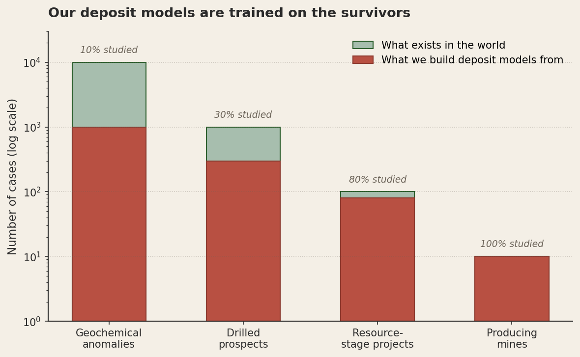
This matters when we build deposit models. A deposit model is, more or less, a description of the diagnostic features that distinguish "real" deposits from background noise. We extract those features by looking at known deposits and asking what they have in common. The trouble is that "known deposit" is the most filtered category in the entire dataset. Every economic deposit in the textbook had to (a) form, (b) be preserved, (c) be near enough to the surface or to inhabited country to be discovered, (d) be discoverable with the technology available at the time, (e) have grade and tonnage that justified development, (f) attract the capital to be developed, and (g) survive long enough to be written about. Each of those filters is multiplicative. The set of deposits that pass all seven is a tiny, weird sample.
What we call "the diagnostic features of porphyry copper systems" might really be "the diagnostic features of the porphyry systems that were big enough, near-surface enough, and outcrop-friendly enough to be found and developed in the last hundred and fifty years." Those are not the same thing. The features we treat as essential might just be the features that make a deposit easy to find. A deposit under three hundred metres of post-mineral cover, in a country with poor infrastructure, with a 0.4 percent grade, would be every bit as real as the ones in our training set. It would just be invisible to our sampling mechanism, which is the same as not existing, for purposes of our model.
The machine-learning version is the same problem with more pixels
This is the part that should make anyone training a prospectivity model nervous. A modern ML pipeline takes geological, geophysical, and geochemical data over a province, takes the locations of known deposits as positive examples, and learns a function that distinguishes "looks like a known deposit" from "looks like background." The model is then applied to under-explored ground to flag new targets.
The problem is that the labels are the survivors. The model is not learning what a deposit is. It is learning what a discovered deposit is. The two classes might overlap a lot, but they are not the same set, and the difference is exactly the set of features that made a deposit visible to historical exploration. If your model loves deposits with strong magnetic signatures and shallow oxide caps, you should ask whether the deposit class genuinely requires these things or whether you have just learned the discoverability function. Under cover, in new terranes, with new geophysical methods, that learned function will mislead you in ways that look like good predictions until you drill and find nothing.
The honest version of this model includes negative cases that are as hard as the positives. Drilled prospects that returned nothing are gold-standard negatives. Anomalies that turned out to be barren are nearly as good. Untested ground is the worst kind of negative because you don't actually know it's negative; you only know nobody has looked. A model trained on "deposits versus untested ground" learns to find things that look like deposits in places where nobody has looked, which is interesting, but not the same as finding actual deposits.
Where else this lives in geoscience
Once you start looking, the highway is everywhere. A few quick examples that bite in everyday geoscience work:
Outcrop bias. Resistant lithologies are the ones that stick up out of the regolith. Recessive units are covered by soil, vegetation, or younger sediments. The mapped stratigraphy of any province skews toward what erodes slowly. The chemistry, age, and structural history we know best is for the units that survived weathering long enough to be sampled. The recessive units are still there. They just don't pass through our sampling filter.
Core recovery. Competent rock comes up the hole intact. Fractured, gougy, or clay-altered intervals come up as mush, voids, or lost sections. Your logged drillhole is a survivorship-biased description of the actual rock. The most interesting intervals — fault zones, alteration halos, mineralised structures — are systematically the ones you have least reliable data for, because their physical properties are exactly what makes them poor at surviving the drilling process.
Published intercepts. A drillhole gets reported in a paper if it hit something interesting. The published distribution of intercepts is wildly inflated above the underlying population of holes drilled. If you train your intuition on what you read in the literature, your sense of "what a typical drilling program looks like" is calibrated to the highlight reel.
Memory. The holes you remember from your career are the discovery holes and the spectacular failures. The hundreds of grey, ambiguous, vaguely interesting holes that made up the bulk of the actual work fade. Your mental training set is heavily weighted toward extremes. When you reason from experience, you are reasoning from the tails of the distribution, which is exactly the same problem as the highway.
What to do about it
You cannot will yourself out of survivorship bias any more than you can will yourself into noticing the drivers going your speed. The filters are baked into how the data reaches you. But you can change what you do once you know they're there.
Name the filter that produced your dataset. Before you analyse anything, write a sentence that begins "the only way a sample got into this dataset was…" and finish it. If your sentence is "the sample exists in the geological record," your filter is mild. If your sentence is "someone drilled the hole, recovered the core, logged it, sent it to a lab, the lab returned a result, the project was active long enough to compile it, and someone published or archived the data," your filter is many-stage and severe. The longer the sentence, the more your dataset is the highway from your driver's seat.
Hunt for the missing class. Wald's move was not "be cleverer about the planes you have." It was "the planes I don't have are the data I need." For your prospectivity model, the missing class is the drilled prospects that came up empty. For your deposit model, the missing class is the deposits in poorly explored terranes. For your stratigraphy, the missing class is the recessive units between the ridges. Spending a day finding good negatives is often worth more than spending a week refining what you already have.
Be suspicious of features that are also discoverability features. Magnetic signature, surface geochemistry, oxide cap thickness, structural exposure: all of these are real geological properties of deposits, and all of them are also reasons deposits get found in the first place. A model that loves them might be learning real geology, or it might be learning the search history. Test by holding out deposits that were found in unusual ways (under cover, by accident, by drilling for something else) and see whether your model still finds them.
Ask what the world would look like if your hypothesis is wrong. The drivers going your speed exist regardless of whether you notice them. The deposits under cover exist regardless of whether your model finds them. If your hypothesis is "deposits like X are rare," ask what would have to be true for them to instead be common but undetected. If the answer is "they would have to look exactly like the deposits I can't see," your "rare" might just be your detection threshold.
The cognitive shape of survivorship bias is that the missing data feels like nothing, and the present data feels like everything. The fix is not to feel differently about it. The fix is to keep a list of the things your particular filter excludes, and to treat that list as part of your dataset. The drivers going your speed are out there. They are not your problem to count, but they are part of the road.
This post is part of a series on statistical pitfalls in geoscience, drawn from a talk given at GACMAC 2026.