// statistics for geoscientists

Optimal Stopping: How the 37% Rule Was Discovered, Then Proved

July 28, 2026

In 1611, Johannes Kepler began the search for a second wife. Over the next two years he interviewed eleven candidates. He worked through the whole list, then went back and married number five, a move the eventual theory would not allow. He told his correspondents the search was wearing him out, that he was exhausted by the misery of comparing candidate after candidate. He could not have known he was running an early version of one of the most studied problems in applied mathematics. He could not have known that his pick was, by a happy accident, almost exactly the one the optimal strategy points to. The math that explains why wouldn't be settled for another three and a half centuries.

The shape of the problem

Strip Kepler's situation down to its bones. You will see a sequence of candidates, one at a time. After each one, you must decide whether to accept (in which case the search ends) or reject (in which case the candidate is gone forever and you must look at the next one). You don't know in advance how good the candidates are, only how each compares to the ones you've already seen. You want to maximise the probability of picking the very best one in the entire sequence.

This is the structure of a thousand decisions outside of marriage. Hiring: candidates arrive over weeks; you make an offer or pass. Property acquisition: you tour available leases one at a time; you commit or move on. Drill targets: you score prospects in order; the budget runs out at some point. Buying a house, picking an apartment to rent, choosing a graduate school. Anything where you face a sequence of options, can't go back to the ones you turned down, and want to choose the best.

The naive strategies are all bad. Pick the first one: 1/n probability of being right. Pick the last one: 1/n. Pick the middle one: 1/n. Pick a random one: 1/n. None of these uses the only information you have, which is how each candidate compares to the previous ones.

The optimal strategy uses that information cleanly. Look at the first r candidates without picking any of them; these form a "calibration" set. Then start picking. From candidate r+1 onwards, accept the first one that beats everyone in the calibration set. If you reach the end without finding such a candidate, take the last one. The only question is what r should be.

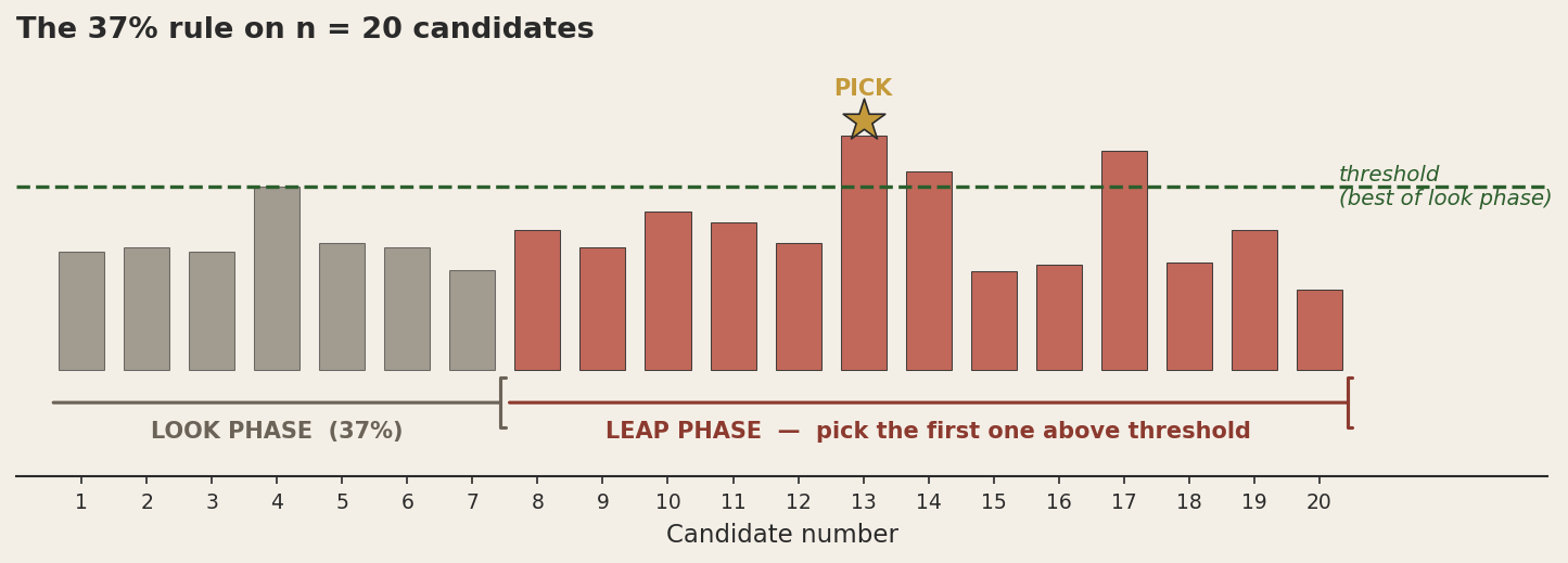
For a sequence of 20 candidates the look phase is 7 (about 37%). The first leap-phase candidate that exceeds the calibration high becomes the pick. Sometimes you find them early. Sometimes you find them late. Sometimes the best candidate is in the look phase and you reject them, never to find another. The strategy is not a guarantee. It is a probability maximiser.

How it became a problem people argued about

Kepler is the colour story, but the actual mathematical lineage starts later. Arthur Cayley, the Cambridge mathematician, posed a problem in 1875 that has the same shape: a person looks at lottery tickets one at a time, must keep one, and cannot retrieve a ticket they've discarded. Cayley computed the expected payoff for some specific cases but didn't generalise.

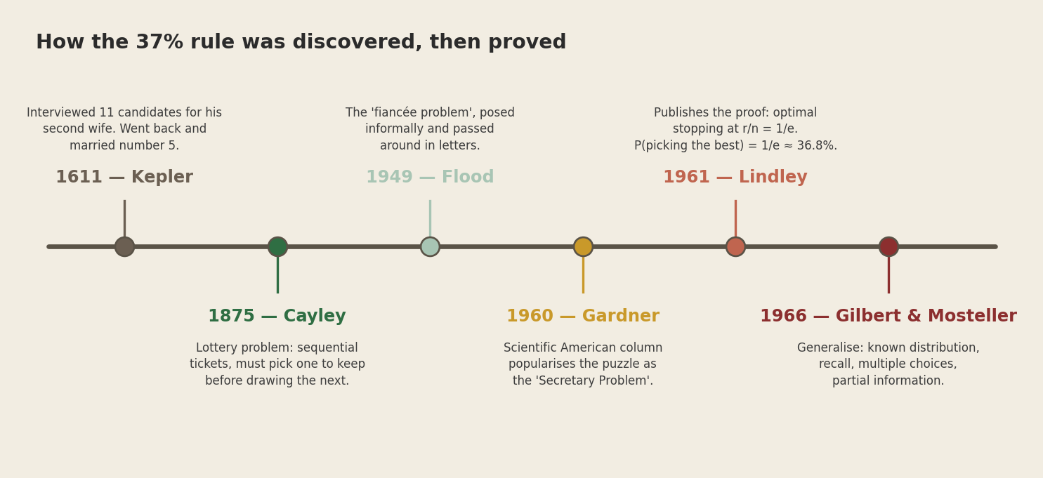
The modern version of the problem was posed informally by Merrill Flood around 1949. Flood, a mathematician at the RAND Corporation and one of the people present at the birth of game theory, called it "the fiancée problem" and discussed it in a letter to colleagues. The problem percolated through the mathematical community in coffee-hour conversations for the next decade.

It became famous in February 1960, when Martin Gardner introduced it to a much wider audience in his Mathematical Games column in Scientific American. Gardner had a knack for picking puzzles whose statements were ten lines long but whose answers were both surprising and beautiful. The fiancée problem, recast as the secretary problem, was perfect for his column. By the time Dennis Lindley published the rigorous proof in 1961, an entire community of mathematicians and statisticians was already working on it. Gilbert and Mosteller generalised it in 1966 to the case where you can recall earlier candidates, the case where you know the underlying distribution, and several other variants. The literature has grown ever since.

The proof, in slow motion

Here is the part of the post I most wanted to write, because the math has the kind of elegance that's worth slowing down for.

You have n candidates in a sequence. The strategy is: reject the first r, then accept the first one (from position r+1 onward) that beats everything in the first r. If you reach the end of the sequence without finding one, take the last one (this rarely matters in the asymptotic analysis).

What is the probability that this strategy picks the single best candidate? Call that probability P(r).

The trick is to condition on which position the best candidate occupies. The best candidate is, with probability 1/n, in any given position. Let's condition on it being in position k. Then:

• If k ≤ r: the best candidate is in the calibration set, gets rejected, and we never find them. Probability of success: 0.
• If k > r: the best candidate is in the leap phase. We will pick them provided nobody before them in the leap phase has been picked first. The previous-best of positions 1 through k-1 must lie in positions 1 through r (otherwise we would have stopped on it). The probability that the previous-best of any k-1 randomly arranged elements happens to lie in the first r of them is exactly r/(k-1).

So the probability of picking the best candidate, given they're in position k, is:

P(success | best in position k) = r / (k-1)   for k > r,   0 otherwise.

Summing over all positions, weighted by 1/n:

P(r) = (1/n) · Σk=r+1n r/(k-1) = (r/n) · Σj=rn-1 1/j

The sum of 1/j from r to n-1 is a partial harmonic sum, well approximated by the natural log of n/r when both are large. So for big n:

P(r) ≈ (r/n) · ln(n/r)

This is the function we want to maximise. Substituting x = r/n (the look-phase fraction):

f(x) = x · ln(1/x) = −x ln x

Take the derivative and set it to zero:

f'(x) = −ln(x) − 1 = 0  ⇔  ln(x) = −1  ⇔  x = 1/e

The optimal look-phase fraction is exactly 1/e ≈ 0.3679. And the maximum probability of success is:

f(1/e) = (1/e) · ln(e) = 1/e ≈ 0.3679

So you look at 1/e of the candidates, and you get a 1/e chance of picking the best. The symmetry is what makes this such a satisfying problem.

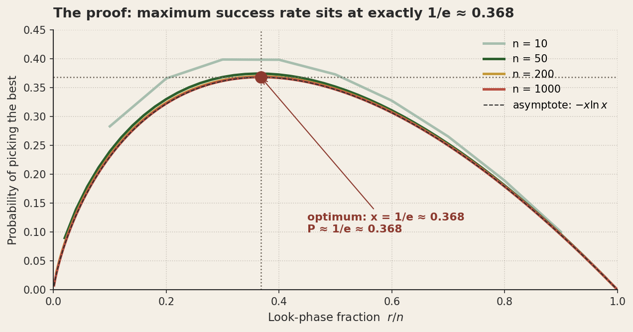
One thing I love about this curve is how flat it is near the optimum. You don't need to hit exactly 37%. Anywhere from about 30% to 45% gives you nearly the same success probability. The 37% number is the one that gets the headlines, but in practice, "look at about a third, then start picking" is almost as good as the precise rule, and it generalises better when the assumptions of the model are violated.

What the rule assumes, and why those assumptions matter

The 1/e proof requires four assumptions. They're worth listing because real decisions almost never satisfy all four.

You see candidates one at a time, in random order. If the order is non-random (best ones tend to come first, say, because the recruiter pre-sorts the résumés), the rule's calibration is off. With a known bias, you can compute a different optimal r; for many natural biases the answer is to look at fewer than 37%.

You can compare any two candidates and decide who's better. The proof only uses ordinal comparisons, not absolute scores. If you have absolute scores from a known distribution, you can do better than 1/e (Gilbert and Mosteller, 1966), often much better.

You must commit at the moment you reject. No going back. If you can recall earlier candidates with some probability of acceptance, the optimal strategy changes and the success probability rises. In real hiring, you can often go back, and most hiring committees do something between "no recall" and "free recall." (Kepler went back for number five, so he was solving the recall variant all along.)

You only care about getting the absolute best. If you'd be happy with a top-three candidate, the optimal strategy looks different. With "happy with top 25%" as the goal, the look-phase fraction should be much smaller, because you can leap earlier and still hit your target.

This is the place where I have to be honest about applying the secretary problem to real-world decisions. Most real decisions violate at least two of these assumptions. That doesn't make the math useless. It makes it a starting point: a clean, exactly-solvable model whose deviations from real situations you can analyse one at a time. The number 37% is often not the right number for your specific problem, but the structure of "calibrate first, then commit" almost always is.

Applied to mineral exploration

Most mineral exploration decisions live one or two steps removed from the secretary problem. Here are a few translations.

Property generation. You evaluate properties one at a time over a season; budget runs out at some point. The structure of "look at the first third without committing, then strike on the first one that beats your calibration" is genuinely useful. It is easy to commit too early or too late here. I have watched both, and either failure mode is expensive.

Drill target selection. If you have a hundred prospectivity-ranked candidates and budget for thirty drill holes, the secretary problem is the wrong model, because you can drill multiple targets and you have absolute scores rather than only ordinal ones. The right model is multi-armed bandit theory, where strategies like upper-confidence-bound (UCB) and Thompson sampling outperform pure greedy ranking. Both are explicitly designed to balance exploitation (drill the high-score targets) with exploration (drill some uncertain ones to learn).

The connection to the 37% rule is conceptual, not numerical. Both come from the same family of "explore-then-exploit" mathematics. The secretary problem is the cleanest case (one-shot, ordinal, no-recall), but the principle that you should sometimes deliberately not pick the best-looking option, in order to learn something useful, is universal across the family. Pure greedy strategies are almost always suboptimal in problems with uncertainty.

The "explore vs. exploit" trade-off in your career. You can spend a season working on a known target type, in a known terrane, where your model says you'll find moderate-value mineralisation. Or you can spend a season working on a novel target type, in an under-explored terrane, where your model has weak predictions but the upside, if you're right, is much larger. Which you choose depends on where you are in your career. Early on, the balance tips toward exploring. Later, it tips toward exploiting what you already know. The reasoning comes from the same explore-then-exploit family as the 37% rule.

The deeper lesson

The thing the secretary problem teaches, beyond the specific 37% number, is that there is a kind of decision-making where the cost of perfectionism is bigger than the cost of a slightly imperfect choice. If you keep waiting for "the best" candidate, you will, with high probability, pass on them in the calibration phase and never find them. The 37% rule is a way of saying: yes, you will sometimes pass on the best candidate, but in expectation, the strategy of looking and then leaping does better than any strategy that waits longer.

I think this is one of the few areas of applied mathematics that has genuinely changed how I make decisions. Faced with a sequence of options, I now try to identify two things explicitly: how many am I going to see, and what is my "look phase" before I start committing? These are not always answerable, but the act of asking them clarifies the decision in ways that just "I'll know it when I see it" does not. The question "have I seen enough yet to know what good looks like?" is one of the most useful questions I know.

Kepler, in 1611, did not know that number five of eleven was within a hair's breadth of the pick the optimal rule prescribes, for a problem that wouldn't be solved until 1961. He just got married, then went on to discover the third law of planetary motion. The marriage, by the way, lasted until his death in 1630 and was reportedly happy. The 37% rule had time on its side.