
The Law of Small Numbers: When n=12 Is Just a Rumour
Here is a real result that has been replicated more times than it should need to be. If you rank U.S. counties by their incidence of kidney cancer, the highest-rate counties are overwhelmingly rural, sparsely populated, and concentrated in the South and Midwest. The first time you see this, you will start building a story. Maybe it's the diet. Maybe it's poor access to early diagnosis. Maybe it's pesticides on farmland. The story is reasonable, the data is real, but the reasoning is off.
It is wrong because if you flip the question and ask which counties have the lowest kidney cancer rates, you find, again, that they are overwhelmingly rural, sparsely populated, and concentrated in the South and Midwest. Both ends of the distribution come from the same set of counties. Whatever your story for the high-rate counties has to be, it has to also explain why those exact same counties are simultaneously the least dangerous places to live. No story does. There is no story to be told here at all. There is only the law of small numbers.
What the law actually says
The law of large numbers, commonly learned in undergrad stats, says that as your sample size grows, your sample mean converges on the true population mean. Flip a fair coin a thousand times and the proportion of heads will be very close to half. Flip it ten times and you might get seven heads and feel surprised, but ten is just not enough flips to feel anything about. This is an old result, and most people accept it.
The "law of small numbers" is a phrase Tversky and Kahneman used semi-ironically to point out that the people who confidently believe in the law of large numbers don't seem to apply it in the other direction. We all know that small samples have more sampling variance than large ones. We don't actually act as if small samples have more variance. We treat n=12 with the same epistemic confidence as n=12,000, and then we are routinely surprised when the small-sample result fails to replicate.
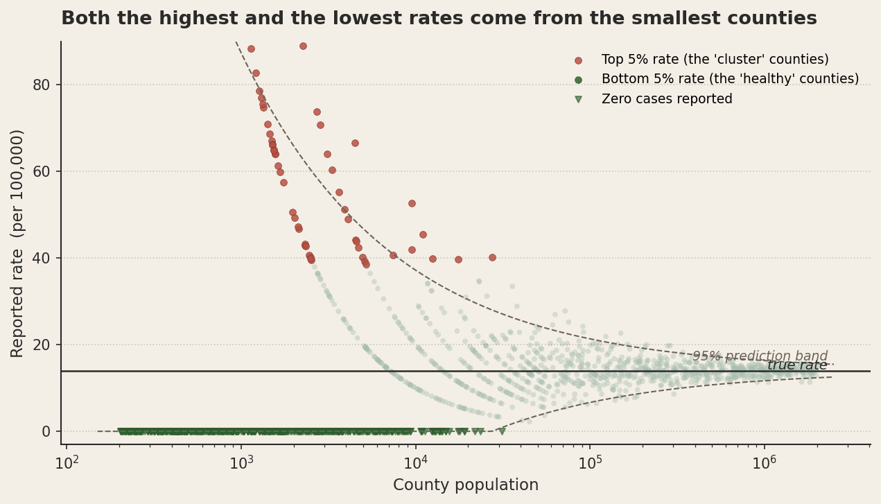
The kidney cancer pattern is the funnel above. Small counties produce extreme rates in both directions, because in a county of five hundred people, a single case of kidney cancer translates into a rate of two hundred per hundred thousand, while zero cases translates into a rate of zero. There's no smooth gradation possible at small N. You either have the case or you don't, and either outcome looks dramatic compared to the smoothed-out rate of a metropolitan county. The rural counties don't have unusual underlying rates. They have unusual observed rates, because the law of small numbers gave them a wide sampling distribution to draw from.
This is the funnel-plot shape that anyone who has worked in epidemiology, manufacturing quality control, or institutional rankings knows on sight. Test scores by school, with school size on the x-axis: same shape. Surgeon mortality rates by case volume: same shape. Mutual fund returns by years of operation: same shape. Anywhere a rate is computed from a count, and the count is small, the rate is mostly noise.
Where this lives in geochemistry
The reason this matters for exploration is that we routinely make decisions based on samples that are way too small to support them, and we don't usually do the bootstrap to find out. The classic case is the orientation survey. You take twelve stream sediment samples around a known prospect, you compute a Cu/Zn ratio, you see that it's about twenty-five percent above your assumed background, and you decide the area shows an anomalous geochemical signature. Sometimes, this is all you have to go on, which is fine. But this concept should always be in the back of your mind.
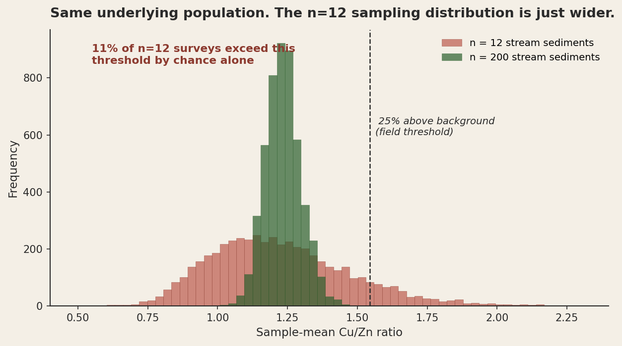
The bootstrap on this is brutal. If you simulate sampling twelve points repeatedly from a single, completely homogeneous background population, more than ten percent of those samples will land above the "twenty-five percent above background" threshold. By chance. With nothing geological happening at all. Your "anomaly" is not impossible to be real, but it is also entirely consistent with you having drawn the wrong twelve samples from a featureless province. The signal-to-noise ratio at n=12 is just too low to distinguish real enrichment from sampling variance.
The version that bites is when this orientation survey then becomes the basis for a much larger and more expensive program. The follow-up four-hundred-sample grid comes back showing background levels everywhere, and the team is confused. The data is internally consistent. The program is not at fault. The orientation survey was a draw from a wide distribution, and the follow-up program is a draw from the same population at much higher N. The follow-up regresses, in exactly the same shape as the kidney cancer funnel narrows toward true rate as county population grows.
What gets lost in the funnel
The harder version of this problem is the one I think doesn't get talked about enough. It is not just that small-N anomalies sometimes turn out to be noise. It is that the entire structure of how we generate exploration leads is biased toward small-N evidence, because small-N evidence is what produces extreme observations, and extreme observations are what get our attention.
If you are running a big systematic survey, your n is large, your variance is small, and you are not going to find anomalies that are statistically dramatic. You will find ones that are real but unimpressive. Meanwhile, somebody on the next lease over has done a half-day reconnaissance with twelve samples and is reporting numbers four hundred percent above background. Their finding is loud, dramatic, and almost certainly mostly noise, but it sounds more exciting than your careful, low-variance, well-bounded estimate. Funding follows the loud number. The entire ecosystem rewards small-N reports because they have wider distributions and therefore generate more attention-grabbing extremes.
This is structurally identical to the medical literature problem of underpowered studies. Small studies that are positive get published, in part because they have to make extreme claims to clear significance thresholds at low N. Their effect sizes are inflated by the very fact of having survived the publication filter at small N. When the well-powered replication eventually arrives, the effect is much smaller, often zero. This is the medical literature's "replication crisis," and the geoscience literature has its own quieter version of the same dynamic.
The thing about means and the thing about ratios
One subtlety worth flagging, because it bites people who have internalised the law of large numbers but apply it loosely. The law of large numbers tells you that the sample mean converges on the true mean as N grows. It does not tell you that any particular sample value is predictable. If your distribution has a heavy right tail, even at large N you can still have wild individual observations. The law tames the average. It does not tame the data.
Geological data is famously heavy-tailed. Grade distributions in many deposits are roughly log-normal. A handful of high-grade samples can pull the mean dramatically. With low N, those high-grade samples either show up (and your mean is dramatically high) or they don't (and your mean is dramatically low). Either way, the sample mean is a poor estimator of the underlying mean grade, because the distribution it's sampling from has the kind of tail that the mean is sensitive to. The fix is to use medians, or to log-transform before averaging, or to model the tail explicitly. The law of large numbers will eventually deliver you the right answer, but "eventually" can be a much larger N than you have budget for.
Ratios are even worse. The Cu/Zn ratio in my simulated stream sediments above behaves badly at small N, in part because it's a ratio of two random variables. Ratios concentrate the variance of both the numerator and the denominator into a single statistic. A small denominator, easily achieved at small N, produces wild ratio values. The "anomalous" element ratio is one of the most overinterpreted statistics in the geochemical toolkit, because the ratio amplifies whatever sampling noise is already in the underlying concentrations.
What to actually do
You can't will yourself out of the law of small numbers any more than you can will yourself into making n=12 behave like n=1000. But you can change your defaults.
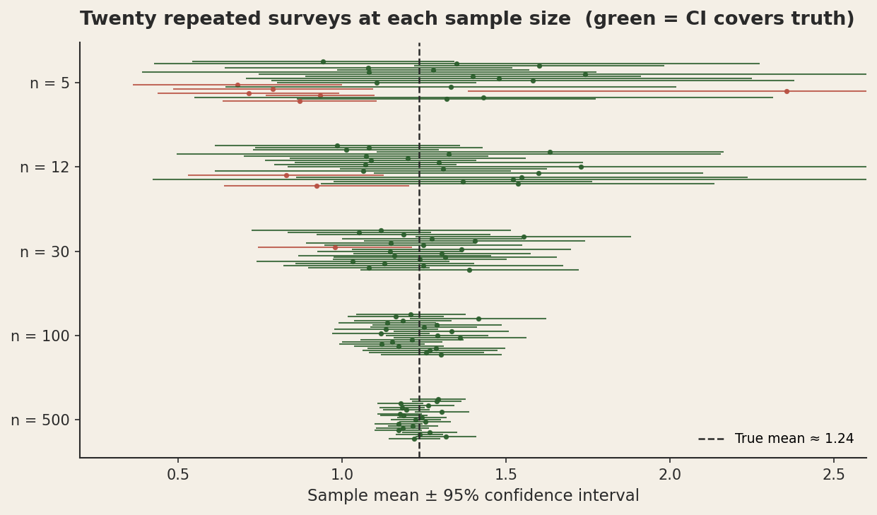
Compute the bootstrap before you celebrate. Take your sample, resample it with replacement a few thousand times, compute the statistic of interest each time, and look at the resulting distribution. The 95 percent confidence interval on a small-N statistic is almost always wider than the analyst's intuition expects. If the confidence interval includes "no anomaly," your point estimate doesn't get to claim "anomaly" without qualification.
Show the funnel. When you publish a regional summary that compares per-property anomaly intensities or per-target prospectivity scores, plot them against the number of samples that went into each estimate. If the small-N properties dominate the top of your ranking, you are looking at the small-N noise more than you are looking at geology.
Anchor the threshold to the sample size. A "twenty-five percent above background" threshold means very different things at n=12 and n=500. The N=500 version, if you cross it, is informative. The N=12 version is barely worth raising. You can build an N-aware threshold that scales the required effect size by the standard error, which is exactly what every formal hypothesis test does, but which most field geochemistry never gets around to.
Remember that "no signal" is also a finding. The funnel is symmetric. Just as small-N surveys produce false anomalies, they also produce false reassurances. A twelve-sample reconnaissance that comes back at background is evidence for "no anomaly here" only at the same low confidence as the anomalous version. Programs sometimes get killed on the basis of small-N negatives, and the law of small numbers is just as merciless to that decision as to the symmetric one.
Be especially suspicious of ratios. If your headline finding is a ratio (Cu/Zn, La/Y, REE-something/REE-something, isotope ratios, alteration indices), bootstrap the ratio not the components. Ratios behave badly at small N in ways that the underlying concentrations don't, and the ratio's confidence interval is often dramatically wider than you'd guess by inspection.
The kidney cancer counties are not strange. They are a perfectly straightforward consequence of how variance behaves at small N. The same shape is in your stream sediment survey, your half-dozen step-outs, your assay batch from one lab vs another, and any time you take a small sample and compute a statistic from it. The number is real. The question is how much of it is the population you sampled and how much of it is the way the law of small numbers shapes the sampling distribution. With n=12, the answer is almost always: more than you'd like to admit.
This post is part of a series on statistical pitfalls in geoscience, drawn from a talk given at GACMAC 2026.